Explore a Kaggle dataset with an in-memory, analytical SQL database. Utilize a ‘best-of-both-worlds’ hybrid Python and R environment.
1 Dataset Context
The grounds for analyses in this case is the problematic behavior as it pertains to the subjects’ experience and their parents’ via questionnaires, physical fitness tests, worn instrument measurements and demographics. The resulting data is to be processed and connections drawn. (Santorelli et al., 2024)
This is a means to apply formatting to every column in a table using a desired paletteer palette if desired using the gt tables. Table output were customized to a high degree. Some functional programming, in particular, are implemented here as they seem to be most appropriate to achieve the desired effect. (Iannone et al., 2025)
Iannone, R., Cheng, J., Schloerke, B., Hughes, E., Lauer, A., Seo, J., Brevoort, K., & Roy, O. (2025). Gt: Easily create presentation-ready display tables. https://gt.rstudio.com
The following R script defines two functions, eval_palette and r_table_theming, which work together to create and style a table using the gt package. The table is customized with colors, headers, footnotes, and other visual elements.
Features:
Dynamic Palette Evaluation: The eval_palette function is flexible and supports multiple palette types, making it reusable for different visualization needs.
Iterative Styling: The use of reduce to iteratively apply styles and footnotes is a clean and efficient approach, especially for tables with many columns or complex styling requirements.
Customizability: The function allows for extensive customization, including font sizes, multiline footnotes, and targeted column coloring.
Here are some relatively simpler functions developed with the intention to append and apply consistent theming to ggplots. R libraries are currently preferred for plotting outputs as they can be extensively customized. (Wickham, 2016)
Wickham, H. (2016). ggplot2: Elegant graphics for data analysis. Springer-Verlag New York. https://ggplot2.tidyverse.org
The data was imported from Kaggle. It only needed to be done once, so the code chunk’s eval setting is set to false during most of this project’s development.
Executed once to import the data from the Kaggle server.
Extracting the downloaded files was also done programmatically, but it is not necessary. It did seem useful to visualize the data directory following extraction to verify the files and folders that now exist in the ./data directory of this project.
Extracted the compressed files and list files.
from zipfile import ZipFileimport pandas as pdzip_path ="child-mind-institute-problematic-internet-use.zip"ifnot os.path.exists('./data/train.csv'):with ZipFile(zip_path) as zf: ZipFile.extractall(zf, path ='./data')print("Extracted files", sep ="\n"*2)else:print("Files already exist", sep ="\n"*2)
Files already exist
Extracted the compressed files and list files.
extracts = pd.DataFrame( data = os.listdir(path ='./data'), columns = ['./data'])
An in-memory, DuckDB database connection was established for this project. The analysis in this project heavily relies on SQL syntax, and most of the computations are performed in database for efficiency.
Set up an in-memory database.
import duckdbconn = duckdb.connect(':memory:')
3.1 Customize Database Settings
Set the database memory limit.
try: conn.sql(f"SET memory_limit = '24GB';")print(f"Successfully changed memory limit to 24GB")except:print(f"An error occurred in changing the memory limit.")
Successfully changed memory limit to 24GB
Set the default ordering for the database.
try: conn.sql(f"SET default_order = 'ASC';")print(f"Successfully changed the default order to ascending.")except:print(f"The default order could not be changed.")
Successfully changed the default order to ascending.
4 Setup Database
4.1 Create New Data Types
Enum data types significantly sped up many database operations. Enums are similar to the category data type in Python, and the factor datatype in R. (Holanda, 2021)
This is designed to manage ENUM types in a DuckDB database in a modular and user-friendly way. It provides functions to create and drop ENUM types, and it uses Python data structures like pandas Series and dictionaries to handle inputs and outputs.
It is part of the data preprocessing and database setup pipeline in this project. It ensures that the database schema (specifically ENUM types) is properly configured before performing further operations, such as aggregating light exposure data.
An approach for defining and verifying custom data types in the database.
def try_create(conn,type_str: str, enum_str: str) -> pd.Series:""" :::WHY(s)::: Is there a modular approach to creating ENUM types in a database? :::HOW(s)::: Utilize python data structures such as pandas Series and dictionary as parameters. """# the try, except can help categorize the outputs for ui/uxtry: conn.execute(f"CREATE TYPE {type_str} AS ENUM {enum_str};")return pd.Series(type_str, index = ['created'])except duckdb.duckdb.CatalogException:return pd.Series(type_str, index = ['already existed'])def try_drop(conn, type_str: str) -> pd.Series:""" :::WHY(s)::: Is there a modular approach to dropping ENUM types in a database? :::HOW(s)::: Utilize python data structures such as pandas Series and dictionary as parameters. """try: conn.execute(f"DROP TYPE {type_str};")return pd.Series(type_str, index = ['dropped'])except duckdb.duckdb.CatalogException:return pd.Series(type_str, index = ['did not exist'])droplist = []for e in enums: droplist.append(try_drop(conn, type_str = e))dropFrame = pd.DataFrame(droplist)dropFrame = dropFrame.sort_values(by = dropFrame.columns.to_list(), ascending =True, ignore_index =True)createList = []for eType, eSeries in enumDict.items(): createList.append(try_create(conn, type_str = eType, enum_str = eSeries))createFrame = pd.DataFrame(createList)createFrame = createFrame.sort_values(by = createFrame.columns.to_list(), ascending =True, ignore_index =True)pydf = pd.concat([dropFrame, createFrame], axis =1)
table setup
r_df <- py$pydfif (colnames(r_df[1]) =="did not exist"){ locations_list =list("did not exist", "created") notes_list =list("Enums that did not exist.","Enums that now exist.") } else { locations_list =list("dropped", "created") notes_list =list("Enums that were dropped.","Enums that now exist.") }# Create a table dataframe, or tibble, of footnotesfootnotes_df <-tibble(notes = notes_list, locations = locations_list)pal_df <-tibble(cols = locations_list,pals =list(eval_palette("ggsci::legacy_tron", 7, 'd', 1)) )#tbl_font_size = pct(80))rTable <-r_table_theming(r_df,title ="Custom Data Types",subtitle =NULL, footnotes_df,source_note =md("**source**: Kaggle"), pal_df,multiline_feet =TRUE,tbl_font_size =pct(80) )
Table 2: Enums dropped and created.
Custom Data Types
did not exist1
created2
age_enum
age_enum
disease_risk_enum
disease_risk_enum
enroll_season_enum
enroll_season_enum
hour_enum
hour_enum
id_actigraphy_enum
id_actigraphy_enum
internet_hours_enum
internet_hours_enum
minute_enum
minute_enum
pciat_season_enum
pciat_season_enum
quarter_enum
quarter_enum
second_enum
second_enum
sex_enum
sex_enum
sii_enum
sii_enum
weekday_enum
weekday_enum
source: Kaggle
1 Enums that did not exist.
2 Enums that now exist.
4.2 Initial Extraction Transformation and Load Pipeline
Transformations are applied while reading in data from files to minimize steps needed. Not sure why the data had hyphens in the columns names, originally. These hyphens interfere with SQL database queries, so it might be useful to replace them with underscore characters. There is no need to overwrite the original CSV’s to maintain a clear trail of data transformations.
Initial data pipeline extraction, transformation and loading to the database.
def setup_duckdb_pipeline( csvDict: dict, parquetDict: dict, conn: duckdb.DuckDBPyConnection) ->None:try: { table_name: duckdb.sql(f""" CREATE OR REPLACE TABLE {table_name} AS SELECT * FROM df; """, connection = conn) for table_name, df in csvDict.items() }for key, value in csvDict.items(): result = conn.execute(f"SELECT COUNT(*) FROM {key}").fetchone()print(f"Successfully created table: {key}, Row count: {result[0]}")exceptExceptionas e:print(f"Error loading table: {str(e)}")raiseif parquetDict: write_datasets(conn, parquetDict)# Create tables from Parquet filesdef write_datasets ( conn: duckdb.DuckDBPyConnection, parquetDict: dict):try: { table_name: duckdb.sql(f""" CREATE OR REPLACE TABLE {table_name} AS SELECT id::id_actigraphy_enum AS id ,quarter::TEXT::quarter_enum AS quarter ,weekday::TEXT::weekday_enum AS weekday ,light ,(time_of_day / 3_600_000_000_000) AS hour_of_day ,relative_date_PCIAT FROM read_parquet( '{file_path}' ,hive_partitioning = true );""", connection=conn)for table_name, file_path in parquetDict.items() }for key, value in parquetDict.items(): result = conn.execute(f"SELECT COUNT(*) FROM {key}").fetchone()print(f"Successfully created table: {key}, Row count, {result[0]}")exceptExceptionas e:print(f"Error writing dataset: {str(e)}")raisetrainCsvDf = pd.read_csv("data/train.csv")testCsvDf = pd.read_csv("data/test.csv")dictDf = pd.read_csv("data/data_dictionary.csv")trainCsvDf.columns = trainCsvDf.columns.str.replace('-','_') trainCsvDf.columns = trainCsvDf.columns.str.lower() testCsvDf.columns = testCsvDf.columns.str.replace('-','_') testCsvDf.columns = testCsvDf.columns.str.lower() dictDf.Field = dictDf.Field.replace("-", "_", regex =True)csvDict = {"TrainCsv": trainCsvDf ,"TestCsv": testCsvDf ,"DataDict": dictDf }parquetDict = {"ActigraphyTrain": 'data/series_train.parquet*/*/*' ,"ActigraphyTest": 'data/series_test*/*/*' }try: setup_duckdb_pipeline(csvDict, parquetDict, conn)except:print(f"Could not set up data pipeline.")
Successfully created table: TrainCsv, Row count: 3960
Successfully created table: TestCsv, Row count: 20
Successfully created table: DataDict, Row count: 81
Successfully created table: ActigraphyTrain, Row count, 314569149
Successfully created table: ActigraphyTest, Row count, 439726
Verify ActigraphyTrain in the database.
pydf = conn.sql(f"""SELECT *FROM ActigraphyTrainORDER BY id ASC ,relative_date_PCIAT ASC ,hour_of_day ASCLIMIT 10;""").df()
table setup
r_df <- py$pydfr_df <- r_df |> dplyr::select(id, quarter, weekday, relative_date_PCIAT, light, hour_of_day)notes_list =list("Unique participant identifier code, to track related data from actigraphy to hbn datasets.","Annual quarter related to month of observation.","Day of the week (Monday = 1)","Light exposure, measured in 'lux'","24-hour time converted to a float for easier conversion for time-series analysis.","Days since questionairre, also convenient to help order daily values for time-series analysis." )locations_list =list("id","quarter","weekday","light","hour_of_day","relative_date_PCIAT")footnotes_df <-tibble(notes = notes_list, locations = locations_list)pal_df <-tibble(cols = locations_list,pals =list(eval_palette("harrypotter::ravenclaw", 7, 'c', 1)))rTable <-r_table_theming(r_df,title ="Actigraphy Data - Training Set",subtitle =NULL, footnotes_df,source_note =md("**source**: Kaggle"), pal_df,multiline_feet =TRUE#tbl_font_size = pct(85) )
Table 3: A preview of ActigraphyTrain database table.
Actigraphy Data - Training Set
id1
quarter2
weekday3
relative_date_PCIAT4
light5
hour_of_day6
00115b9f
3
4
41
53.00000
15.81667
00115b9f
3
4
41
51.66667
15.81806
00115b9f
3
4
41
50.33333
15.81944
00115b9f
3
4
41
50.50000
15.82083
00115b9f
3
4
41
33.16667
15.89861
00115b9f
3
4
41
31.33333
15.90000
00115b9f
3
4
41
29.50000
15.90139
00115b9f
3
4
41
27.66667
15.90278
00115b9f
3
4
41
25.83333
15.90417
00115b9f
3
4
41
24.00000
15.90556
source: Kaggle
1 Unique participant identifier code, to track related data from actigraphy to hbn datasets.
2 Annual quarter related to month of observation.
3 Day of the week (Monday = 1)
4 Days since questionairre, also convenient to help order daily values for time-series analysis.
5 Light exposure, measured in 'lux'
6 24-hour time converted to a float for easier conversion for time-series analysis.
5 EDA
This is designed to filter and create new database tables based on regular expression (regexp) patterns applied to column names. It is part of the data preprocessing pipeline. The code modularizes the process of selecting columns and creating new tables, making it reusable and efficient.
Creates several tables based on column label strings.
import redef filter_columns_by_regex(col_dict: dict, regex_pattern: str) ->dict:""" :::WHY(s)::: Can there be a way to use dictionaries to specify columns? :::GOAL(s)::: Regex selection of column names from a dictionary. """return { col: dtype for col, dtype in col_dict.items() if re.search(regex_pattern, col) }def create_table_with_regex_columns( conn: duckdb.duckdb ,source_table: str ,new_table_name: str ,regex_pattern: str ,col_dict: dict ) ->None: """ :::WHY(s)::: There should to be a more streamlined way to utilize columnar information following regular string patterns to generate tables based on such information. This could follow and carry out pre-existing data modeling plans. :::GOAL(s)::: To create new database tables with modularized SQL queries generated with the help of regex pattern matching selection. :::EXAMPLE(s)::: The dictionary item: "Demographic": r"^id|^sii|^basic\S+" Would generate a table named 'Demographic' from data with columns for 'id', 'sii' and all columns starting with 'basic' strings. """# filter columns filtered_col_dict = filter_columns_by_regex(col_dict, regex_pattern)# regex column selecting via dict comprehension and vectorized filtering regex_select_sql =f""" CREATE OR REPLACE TABLE {new_table_name} AS SELECT{', '.join([f'"{col}"'for col in filtered_col_dict.keys()])} FROM {source_table}; """ conn.execute(regex_select_sql)# It'd be useful to get the data types for creating a new table of valuescoltype_overview = conn.sql(f""" SELECT column_name ,data_type FROM information_schema.columns WHERE table_name = 'TrainCsv';""").df()# Map the column names with data typescol_dict =dict(zip(coltype_overview.column_name, coltype_overview.data_type))regex_dict_train = {"Demographic": r"^id|^sii|^basic\S+" ,"Physical": r"^id|^sii|^physical\S+" ,"FgVital": r"^id|^sii|^fitness_E\S+" ,"FgChild": r"^id|^sii|^fgc\S+" ,"Bia": r"^id|^sii|^bia\S+" ,"Paqa": r"^id|^sii|^paq_a\S+" ,"Pciat": r"^id|^sii|^pciat\S+" ,"Sds": r"^id|^sii|^sds\S+" ,"InternetUse": r"^id|^sii|^preint\S+" }# There's no Pciat in the test setregex_dict_test = {"DemographicTest": r"^id|^basic\S+" ,"PhysicalTest": r"^id|^physical\S+" ,"FgVitalTest": r"^id|^fitness_E\S+" ,"FgChildTest": r"^id|^fgc\S+" ,"BiaTest": r"^id|^bia\S+" ,"PaqaTest": r"^id|^paq_a\S+" ,"SdsTest": r"^id|^sds\S+" ,"InternetUseTest": r"^id|^preint\S+" }# Loop through the data structures to create tables for the train setfor new_table_name, regex_pattern in regex_dict_train.items(): create_table_with_regex_columns( conn ,'TrainCsv' ,new_table_name ,regex_pattern ,col_dict ) # Loop through the data structures to create tables for the test setfor new_table_name, regex_pattern in regex_dict_test.items(): create_table_with_regex_columns( conn ,'TestCsv' ,new_table_name ,regex_pattern ,col_dict )
Perform a join on matching Ids to combine demographics data with actigraphy data such as time and light exposure.
conn.sql("""CREATE OR REPLACE TABLE IntermediateActigraphy ASSELECT id ,basic_demos_enroll_season::TEXT::enroll_season_enum AS enroll_season ,basic_demos_age::TEXT::age_enum AS age ,basic_demos_sex::TEXT AS sex ,sii::INTEGER::TEXT::sii_enum AS siiFROM DemographicORDER BY id ASC;""")conn.sql("""CREATE OR REPLACE TABLE ActigraphyTrainAS SELECT ia.* ,at.hour_of_day ,at.weekday ,at.quarter ,at.light FROM ActigraphyTrain at LEFT JOIN IntermediateActigraphy ia ON ia.id = at.id;""")conn.sql("""CREATE OR REPLACE TABLE IntermediateActigraphy ASSELECT id ,basic_demos_enroll_season::TEXT::enroll_season_enum AS enroll_season ,basic_demos_age::TEXT::age_enum AS age ,basic_demos_sex::TEXT AS sexFROM DemographicTestORDER BY id ASC;""")conn.sql("""CREATE OR REPLACE TABLE ActigraphyTestAS SELECT ia.* ,at.hour_of_day ,at.quarter ,at.weekday ,at.light FROM ActigraphyTest at LEFT JOIN IntermediateActigraphy ia ON ia.id = at.id;""")conn.sql("DROP TABLE IntermediateActigraphy;")try: conn.sql(f"CHECKPOINT;")print(f"Cleared unused allocated space from memory.")except:print(f"Could not clear from memory.")
┌─────────┐
│ Success │
│ boolean │
├─────────┤
│ 0 rows  │
└─────────┘

Cleared unused allocated space from memory.
5.1 Actigraphy, Physical, and Demographics
It might be useful to explore how the time of day and associated exposure to light might correlate to other factors, such as sii, physical characteristics, and internet use.
5.1.1 Informal Hypothesis
Hypothesis: More time spent indoors on the internet might be associated with lower light exposure during daytime (Q1-Q2, Q2-Q3) and higher light exposure during nighttime (min-Q1, Q3-max).
The BMI risk categories found at, (Zierle-Ghosh & Jan, 2024), have been borrowed for this project. The SQL query syntax, therefore, aims to reflect a structure of evidence-based classification. Though not used in this project, it might be useful to classify lux statistics in a way that reflect a classification standard (Lux Measurements, n.d.).
Repetitive SQL commands are quite verbose and repetitive, at times. Python functions, alongside data structures, such as dataframes, and dictionaries could actually help make running SQL commands less repetitive and more modular.
The code is designed to process and aggregate light exposure data from actigraphy datasets (likely from wearable devices) using DuckDB as an in-memory database. The code is modularized into several functions to handle different tasks, such as calculating quartiles, detecting specific columns, creating intermediate tables, and joining these tables into a final aggregated result.
Additionally, the code is useful for analyzing light exposure data over different times of the day (based on quartiles of hour_of_day). It aggregates the data into meaningful segments and creates a final table that can be used for further analysis or visualization. Included is a try-except block to handle any potential errors during the table joining process, ensuring that the user is informed if something goes wrong.
Extract actigraphy data based on the time of day quartile.
def quartiler( conn: duckdb.duckdb, col_name: str, source_name: str) ->dict:""" ::WHY(s):: SQL can sometimes require a lot of code for repetitive commands, but in a Python environment, database queries can be modularized. ::GOAL(s):: To process SQL queries into useful quartile information represented by intuitive key labels. """ summaryDf = conn.sql(f""" SUMMARIZE SELECT{col_name} FROM {source_name};""").df() quartileDict = {'min': summaryDf['min'][0] ,'Q1': summaryDf.q25[0] ,'Q2': summaryDf.q50[0] ,'Q3': summaryDf.q75[0] ,'max': summaryDf['max'][0] }return quartileDictdef siiDetect (detect_frame: pd.DataFrame) ->bool:if'sii'in detect_frame.column_name.values:returnTruedef intermediateLighter( conn: duckdb.duckdb, new_tables: list, quarters: dict, quartuples: pd.Series, from_table: str) ->None:""" :::WHY(s)::: Tables based on the same parameters but different parameter values could be modularized. :::GOAL(s)::: Process repetitive SQL efficiently and intuitively using data structures that simplify the process. """ detect_frame = conn.execute(f""" SELECT * FROM information_schema.columns WHERE table_name = '{from_table}'; """).df()for i inlist(range(4)):if siiDetect(detect_frame) ==True: conn.sql(f""" CREATE OR REPLACE TABLE {new_tables[i]} AS SELECT id ,enroll_season ,age ,sex ,sii ,AVG(light) AS {quartuples.index[i]} FROM '{from_table}' WHERE hour_of_day BETWEEN {quarters[quartuples.iloc[i][0]]}::DOUBLE AND {quarters[quartuples.iloc[i][1]]}::DOUBLE GROUP BY ALL ORDER BY id ASC;""")else: conn.sql(f""" CREATE OR REPLACE TABLE {new_tables[i]} AS SELECT id ,enroll_season ,age ,sex ,AVG(light) AS {quartuples.index[i]} FROM '{from_table}' WHERE hour_of_day BETWEEN {quarters[quartuples.iloc[i][0]]}::DOUBLE AND {quarters[quartuples.iloc[i][1]]}::DOUBLE GROUP BY ALL ORDER BY id ASC;""")def joinLights (from_to_tables: dict) ->None:for from_table, to_table in from_to_tables.items(): new_tables = ['Light1', 'Light2', 'Light3', 'Light4'] quarters = quartiler(conn, 'hour_of_day', from_table) intermediateLighter(conn, new_tables, quarters, quartuples, from_table) conn.sql(f""" CREATE OR REPLACE TABLE {to_table} AS SELECT l1.* ,l2.q1_q2 ,l3.q2_q3 ,l4.q3_max FROM Light1 l1 LEFT JOIN Light2 l2 ON l1.id = l2.id LEFT JOIN Light3 l3 ON l1.id = l3.id LEFT JOIN Light4 l4 ON l1.id = l4.id; """)for table in new_tables: conn.sql(f"DROP TABLE {table};")quartuples = pd.Series( data = [('min','Q1') ,('Q1', 'Q2') ,('Q2', 'Q3') ,('Q3' ,'max')] ,index = ['min_q1' ,'q1_q2' ,'q2_q3' ,'q3_max'])from_to_tables = {'ActigraphyTrain': 'AggregatedLights' ,'ActigraphyTest': 'AggregatedLightsTest' }try: joinLights(from_to_tables) pydf = conn.sql("SELECT * FROM AggregatedLights LIMIT 10;").df()print(f"Joined the lux tables and saved a preview of the aggregated table.")except:print(f"Lux tables were not joined.")
Joined the lux tables and saved a preview of the aggregated table.
Free unused database memory from dropped tables and such.
try: conn.sql(f"CHECKPOINT;")print(f"Cleared unused memory.")except:print(f"Could not clean unused memory.")
r_df <- py$pydfnotes_list =list("Unique participant identifier.","Participant enrollment into study season.","Age in years.","Sex (0 = Female, 1 = Male)","Severity Impairment Index","Mean light exposure across Q1 of a 24 hour time scale.","Mean light exposure across Q2 of a 24 hour time scale.","Mean light exposure across Q3 of a 24 hour time scale.","Mean light exposure across Q4 of a 24 hour time scale." )locations_list =list("id" ,"enroll_season" ,"age" ,"sex" ,"sii" ,'min_q1' ,'q1_q2' ,'q2_q3' ,'q3_max')footnotes_df <-tibble(notes = notes_list, locations = locations_list)pal_df <-tibble(cols = locations_list,pals =list(eval_palette("harrypotter::ravenclaw", 7, 'c', 1)) )rTable <-r_table_theming(r_df,title ="Quartile Data - Lights",subtitle =NULL, footnotes_df,source_note =md("**source**: Kaggle"), pal_df,multiline_feet =TRUE)
Table 4, returns the averages of light exposure, grouped by individual participants across the 4 6-hour time-frames of the day.
Table 4: Quantiles related to mean lux exposure.
Quartile Data - Lights
id1
enroll_season2
age3
sex4
sii5
min_q16
q1_q27
q2_q38
q3_max9
00115b9f
Winter
9
0
1
23.045631
61.57957
52.81590
17.014504
001f3379
Spring
13
1
1
2.091995
38.87517
27.36520
3.436843
00f332d1
Winter
14
0
1
20.997433
70.66200
172.14445
20.099417
012e3869
Summer
6
0
0
13.294238
21.50671
14.48623
11.505972
029a19c9
Winter
17
1
1
11.332134
58.91847
35.59866
7.528591
02cebf33
Spring
12
1
1
35.523693
21.77969
44.71041
52.702508
02cf7384
Summer
16
1
0
7.042261
21.47413
24.09722
7.120843
035c96dd
Summer
13
1
0
15.085578
16.63144
19.23520
14.558172
0417c91e
Spring
6
1
0
13.857264
132.18453
197.77672
17.241575
04afb6f9
Summer
17
1
2
14.194009
19.53135
19.77159
10.799413
source: Kaggle
1 Unique participant identifier.
2 Participant enrollment into study season.
3 Age in years.
4 Sex (0 = Female, 1 = Male)
5 Severity Impairment Index
6 Mean light exposure across Q1 of a 24 hour time scale.
7 Mean light exposure across Q2 of a 24 hour time scale.
8 Mean light exposure across Q3 of a 24 hour time scale.
9 Mean light exposure across Q4 of a 24 hour time scale.
Join light data with internet use hours data.
lightsDict = {'AggregatedLights': 'InternetUse', 'AggregatedLightsTest': 'InternetUseTest' }for from_tbl, join_tbl in lightsDict.items(): conn.sql(f""" CREATE OR REPLACE TABLE '{from_tbl}' AS SELECT ft.* ,jt.preint_eduhx_computerinternet_hoursday::INTEGER::TEXT::internet_hours_enum AS useHrs FROM '{from_tbl}' ft LEFT JOIN {join_tbl} jt ON ft.id = jt.id; """)
Checking the internet use hours parameter to get an overview along with null percentage to see if we might be able to use it, as-is, for joining with the corresponding lux quartile.
5.1.3 Sii, Lux, and Internet Use
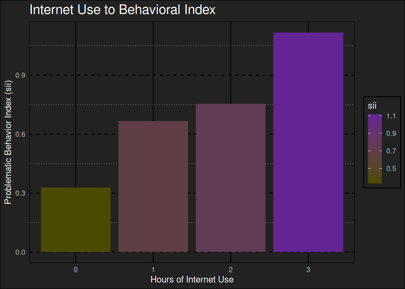
Table 5, is returning some descriptive statistics, such as count and mean, across the behavioral index, and mean lux by quartile, grouped by internet use hours.
Group-averaging sii, internet use hours, and pre-averaged lux quartile by age and sex.
pydf = conn.sql(f"""SELECT useHrs ,COUNT(*) AS observations ,AVG(sii::INTEGER) AS sii ,AVG(min_q1) AS 'q1' ,AVG(q1_q2) AS 'q2' ,AVG(q2_q3) AS 'q3' ,AVG(q3_max) AS 'q4'FROM AggregatedLights alGROUP BY useHrs;""").df()pydf = pydf.dropna()
table setup
r_df <- py$pydfnotes_list =list("Hours spent on the internet, as reported by caregivers of the participants.","Count of observations in the dataset.","Problematic behavior score.","Mean lux (12am to 6am)","Mean lux (6am to 12pm)","Mean lux (12pm to 6pm)","Mean lux (6pm to 12am)" )locations_list =list("useHrs", "observations","sii","q1","q2","q3","q4" )footnotes_df <-tibble(notes = notes_list, locations = locations_list )pal_df <-tibble(cols = locations_list,pals =list(eval_palette("harrypotter::ravenclaw", 7, 'c', 1)) )rTable <-r_table_theming(r_df,title ="Problematic Behavior to Internet Usage",subtitle =NULL, footnotes_df,source_note =md("**source**: Kaggle"), pal_df,multiline_feet =FALSE )
Table 5: Grouped averages of lux to sii.
Problematic Behavior to Internet Usage
useHrs1
observations2
sii3
q14
q25
q36
q47
0
474
0.3291139
12.34923
54.33614
75.33046
14.37498
1
117
0.6666667
15.14069
46.08189
66.78185
15.30225
2
288
0.7534722
14.24140
43.78829
65.41403
15.33504
3
102
1.1176471
18.15549
48.21921
70.29719
19.04650
source: Kaggle
1 Hours spent on the internet, as reported by caregivers of the participants., 2 Count of observations in the dataset., 3 Problematic behavior score., 4 Mean lux (12am to 6am), 5 Mean lux (6am to 12pm), 6 Mean lux (12pm to 6pm), 7 Mean lux (6pm to 12am)
plot setup
library(scales)r_plot <-ggplot(data = r_df, mapping =aes(x = useHrs, y = sii) ) +geom_col(aes(fill = sii)) +scale_fill_gradient(low =muted("yellow"), high =muted("purple")) +labs(title ='Internet Use to Behavioral Index', x ='Hours of Internet Use', y ="Problematic Behavior Index (sii)")r_plot <- r_plot +ggplot_theming()
Figure 1: Categorized bmi risk to internet use and sii.
5.1.4 Disease Risk Categories
Something perhaps not seen everyday is SQL syntax in a Python environment. The performance of the SQL database, in this case, DuckDB, likely outperforms Pandas and Polars. An aim for this project was also to demonstrate some competence with SQL, but also approach practical use-case scenarios.
Combining SQL with Python data structures to organized data according to several conditions, such as: bmi, age, sex, and waist_circumference.
riskyDictionary = {'Risk1': (f",CASE WHEN ph.physical_bmi < 18.5 THEN 'Underweight'" ,f"WHEN ph.physical_bmi BETWEEN 18.5 AND 24.9 THEN 'Normal'" ,f"WHEN ph.physical_bmi BETWEEN 25.0 AND 29.9 THEN 'Increased'" ,f"WHEN ph.physical_bmi BETWEEN 30.0 AND 34.9 THEN 'High'" ,f"WHEN ph.physical_bmi BETWEEN 35.0 AND 39.9 THEN 'Very High'" ,f"WHEN ph.physical_bmi >= 40 THEN 'Extremely High'" ,f"ph.physical_waist_circumference <= 35 AND al.sex = '0'"),'Risk2': (f",CASE WHEN ph.physical_bmi < 18.5 THEN 'Underweight'" ,f"WHEN ph.physical_bmi BETWEEN 18.5 AND 24.9 THEN 'Normal'" ,f"WHEN ph.physical_bmi BETWEEN 25.0 AND 29.9 THEN 'High'" ,f"WHEN ph.physical_bmi BETWEEN 30.0 AND 34.9 THEN 'Very High'" ,f"WHEN ph.physical_bmi BETWEEN 35.0 AND 39.9 THEN 'Very High'" ,f"WHEN ph.physical_bmi >= 40 THEN 'Extremely High'" ,f"ph.physical_waist_circumference > 35 AND al.sex = '0'"),'Risk3': (f",CASE WHEN ph.physical_bmi < 18.5 THEN 'Underweight'" ,f"WHEN ph.physical_bmi BETWEEN 18.5 AND 24.9 THEN 'Normal'" ,f"WHEN ph.physical_bmi BETWEEN 25.0 AND 29.9 THEN 'Increased'" ,f"WHEN ph.physical_bmi BETWEEN 30.0 AND 34.9 THEN 'High'" ,f"WHEN ph.physical_bmi BETWEEN 35.0 AND 39.9 THEN 'Very High'" ,f"WHEN ph.physical_bmi >= 40 THEN 'Extremely High'" ,f"ph.physical_waist_circumference <= 40 AND al.sex = '1'"),'Risk4': (f",CASE WHEN ph.physical_bmi < 18.5 THEN 'Underweight'" ,f"WHEN ph.physical_bmi BETWEEN 18.5 AND 24.9 THEN 'Normal'" ,f"WHEN ph.physical_bmi BETWEEN 25.0 AND 29.9 THEN 'High'" ,f"WHEN ph.physical_bmi BETWEEN 30.0 AND 34.9 THEN 'Very High'" ,f"WHEN ph.physical_bmi BETWEEN 35.0 AND 39.9 THEN 'Very High'" ,f"WHEN ph.physical_bmi >= 40 THEN 'Extremely High'" ,f"ph.physical_waist_circumference > 40 AND al.sex = '1'") }riskyDf = pd.DataFrame(data = riskyDictionary)for key, value in riskyDf.items():try: conn.sql(f""" CREATE OR REPLACE TABLE {key} AS SELECT al.*{value[0]}{value[1]}{value[2]}{value[3]}{value[4]}{value[5]} ELSE NULL END AS risk_cat ,risk_cat::disease_risk_enum AS risk_category FROM Physical ph LEFT JOIN AggregatedLights al ON al.id = ph.id WHERE {value[6]} ORDER BY al.id ASC; """) result = conn.sql(f"SELECT COUNT(*) FROM {key}").fetchone()print(f"created table: {key}, \n\tRow count: {result[0]}\n")except:print(f"Error loading this table: {key}")
created table: Risk1,
    Row count: 24

created table: Risk2,
    Row count: 1

created table: Risk3,
    Row count: 20

created table: Risk4,
    Row count: 2
Combining SQL with Python data structures to organized data according to several conditions, such as: bmi, age, sex, and waist_circumference.
conn.sql(f"""CREATE OR REPLACE TABLE DiseaseRiskDemographic ASSELECT * EXCLUDE(risk_cat) FROM Risk1UNION BY NAMESELECT * EXCLUDE(risk_cat) FROM Risk2UNION BY NAMESELECT * EXCLUDE(risk_cat) FROM Risk3UNION BY NAME SELECT * EXCLUDE(risk_cat) FROM Risk4;""")
It might be useful to explore statistics when grouped by risk categories.
Grouped averaging by risk category.
conn.sql(f"""CREATE OR REPLACE TABLE RiskCategorySummary ASSELECT risk_category ,AVG(sii::NUMERIC) AS sii ,AVG(useHrs::INTEGER) AS useHrs ,AVG(min_q1) AS 'q1' ,AVG(q1_q2) AS 'q2' ,AVG(q2_q3) AS 'q3' ,AVG(q3_max) AS 'q4'FROM DiseaseRiskDemographicGROUP BY risk_category;""")pydf = conn.sql("""SELECT * FROM RiskCategorySummary;""").df()
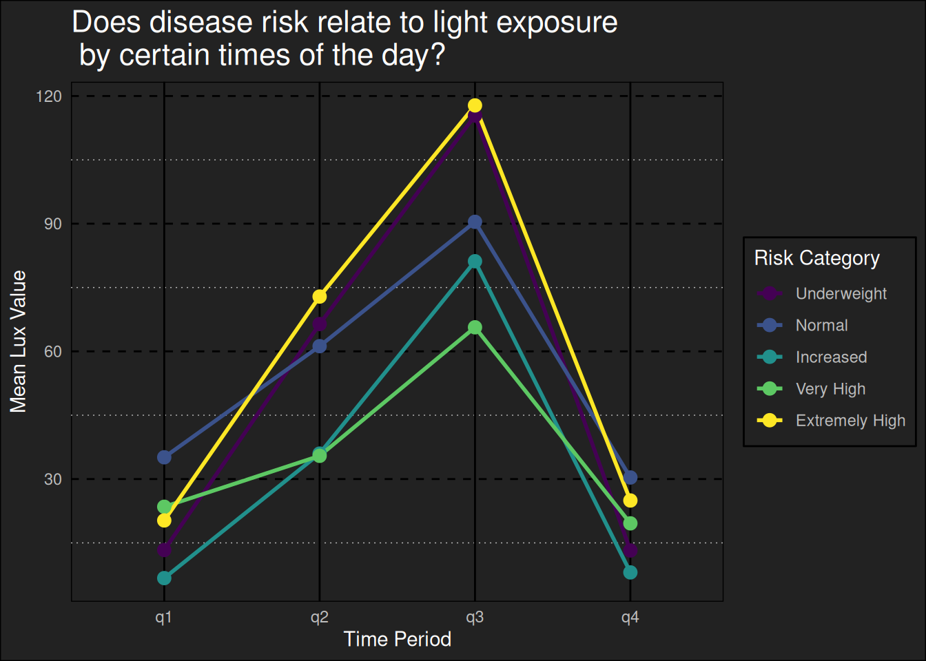
Table 6 shows the grouped-averages of the problematic behavior index, internet use hours, and mean lux across the time of day quartiles by disease risk category of participants.
Table 6: Disease risk categories by lux exposure.
Disease Risk Categories to Lux
risk_category1
sii2
useHrs3
q14
q25
q36
q47
Underweight
0.2424242
0.5757576
13.330039
66.41683
115.40578
13.214609
Normal
0.5000000
1.2000000
35.113050
61.22258
90.43512
30.368059
Increased
0.0000000
2.0000000
6.728299
35.98224
81.17680
8.067938
Very High
0.5000000
2.5000000
23.489066
35.45635
65.65650
19.591619
Extremely High
0.0000000
3.0000000
20.273825
72.87793
117.79320
24.963076
source: Kaggle
1 The disease risk category., 2 Problematic behavior index., 3 Reported interet usage (hours)., 4 12am to 6am, 5 6am to 12pm., 6 12pm to 6pm, 7 6pm to 12am
Pivoting the data longer to accommodate more useful plot output.
locations_list =list("risk_category", "sii", "useHrs", "quarter", "lux")notes_list =list("Disease risk based on BMI, waist circumference, and sex.","Problematic behavior index.","Hours of reported internet use.","Quartile of day.","Average light exposure.")footnotes_df <-tibble(notes = notes_list, locations = locations_list)pal_df <-tibble(cols = locations_list,pals =list(eval_palette("harrypotter::ravenclaw", 7, 'c', 1)))rTable <-r_table_theming(data_long,title ="Disease Risk Categories to Lux",subtitle ="Pivoted Longer", footnotes_df,source_note =md("**source**: Kaggle"), pal_df,multiline_feet =TRUE,tbl_font_size =pct(80) )
Table 7 is a pivoted version of the previous table, Table 6.
Table 7
Disease Risk Categories to Lux
Pivoted Longer
risk_category1
sii2
useHrs3
quarter4
lux5
Underweight
0.2424242
0.5757576
q1
13.330039
Underweight
0.2424242
0.5757576
q2
66.416830
Underweight
0.2424242
0.5757576
q3
115.405777
Underweight
0.2424242
0.5757576
q4
13.214609
Normal
0.5000000
1.2000000
q1
35.113050
Normal
0.5000000
1.2000000
q2
61.222575
Normal
0.5000000
1.2000000
q3
90.435121
Normal
0.5000000
1.2000000
q4
30.368059
Increased
0.0000000
2.0000000
q1
6.728299
Increased
0.0000000
2.0000000
q2
35.982235
Increased
0.0000000
2.0000000
q3
81.176802
Increased
0.0000000
2.0000000
q4
8.067938
Very High
0.5000000
2.5000000
q1
23.489066
Very High
0.5000000
2.5000000
q2
35.456346
Very High
0.5000000
2.5000000
q3
65.656499
Very High
0.5000000
2.5000000
q4
19.591619
Extremely High
0.0000000
3.0000000
q1
20.273825
Extremely High
0.0000000
3.0000000
q2
72.877935
Extremely High
0.0000000
3.0000000
q3
117.793201
Extremely High
0.0000000
3.0000000
q4
24.963076
source: Kaggle
1 Disease risk based on BMI, waist circumference, and sex.
2 Problematic behavior index.
3 Hours of reported internet use.
4 Quartile of day.
5 Average light exposure.
plot setup
r_plot <-ggplot(data = data_long, aes(x = quarter, y = lux, group = risk_category, color = risk_category)) +geom_line(linewidth =1) +geom_point(size =3) +labs(title ="Does disease risk relate to light exposure\n by certain times of the day?",x ="Time Period",y ="Mean Lux Value",color ="Risk Category")r_plot <- r_plot +ggplot_theming()
Figure 2 was an attempt at visualizing the relationship, if any, by mean lux exposure across participants, time of day quartile, and disease risk. Disease risk was based on BMI, waist-circumference, and sex data.
Figure 2: Grouped risk by lux and time period.
6 Summary Profiles
In the future, this data could be further explored. For now, the descriptive statistics can be saved to files for quickly restarting and diving deeper.
Create future training and testing data profiles from summary statistics to inform modeling choices.
summary_dict = {'ActigraphyTrain': ('ActigraphyTrainSummary' ,'data/profiles/actigraphy_train_profile.csv'),'ActigraphyTest': ('ActigraphyTestSummary' ,'data/profiles/actigraphy_test_profile.csv'),'TrainCsv': ('TrainCsvSummary' ,'data/profiles/train_csv_profile.csv'),'TestCsv': ('TestCsvSummary' ,'data/profiles/test_csv_profile.csv') }summary_frame = pd.DataFrame(summary_dict)for key, value in summary_frame.items():try: py_summary_df = conn.sql(f"SUMMARIZE SELECT * FROM '{key}';").df() conn.register(value[0], py_summary_df) conn.sql(f"COPY {value[0]} TO '{value[1]}' (HEADER , DELIMITER ',');")print(f"'{value[1]}' was CREATED\n")except:print(f"'{value[1]}' was not CREATED\n")
<duckdb.duckdb.DuckDBPyConnection object at 0x7b887484d4b0>
'data/profiles/actigraphy_train_profile.csv' was CREATED

<duckdb.duckdb.DuckDBPyConnection object at 0x7b887484d4b0>
'data/profiles/actigraphy_test_profile.csv' was CREATED

<duckdb.duckdb.DuckDBPyConnection object at 0x7b887484d4b0>
'data/profiles/train_csv_profile.csv' was CREATED

<duckdb.duckdb.DuckDBPyConnection object at 0x7b887484d4b0>
'data/profiles/test_csv_profile.csv' was CREATED
7 Close Connection
The in-memory database connection can be closed.
Releases all database memory and de-references the connection variable.
try: conn.close()print(f"database connection closed")except:print(f"could not close the connection")
database connection closed
8 Closing Thoughts
The purpose of the article was to explore an active Kaggle competition dataset and improve workflow methodologies and output. This analysis can be expanded to be more insightful for this particular domain. The objective has been achieved as much was learned and improved functions have been developed alongside improved CSS styling.
This particular dataset contained a lot of missing data despite being quite large. Due to this incomplete data across many of the columns, some of the data transformations resulted in as low as ~50 observations from the original ~1000. The leaderboard that came along with this dataset from a past competition suggests that the model accuracy tops out only around 0.48, Table 8. While some patterns could be gleaned, the predictive power of any modeling attempts might as well have been doomed.
Reads a recently downloaded the private leaderboard csv (from the competition website’s Leaderboard tab) to a dataframe.
r_df <- py$py_dfnotes_list =list("Overall ranking","Unique team ID.","Chosen name of the team.","Their final submission date.","The accuracy score of model.","Total competition submissions.","Names of the team members.")locations_list =list("Rank", "TeamId", "TeamName", "LastSubmissionDate", "Score", "SubmissionCount", "TeamMemberUserNames")footnotes_df <-tibble(notes = notes_list, locations = locations_list)pal_df <-tibble(cols = locations_list,pals =list(eval_palette("ggsci::legacy_tron", 7, 'd', 1)) )rTable <-r_table_theming(r_df,title ="Leaderboard Rankings",subtitle =NULL, footnotes_df,source_note =md("**source**: Kaggle"), pal_df,multiline_feet =FALSE,target_everything =TRUE,color_by_columns ="Rank",tbl_font_size =pct(75) )
Table 8
Leaderboard Rankings
Rank1
TeamId2
TeamName3
LastSubmissionDate4
Score5
SubmissionCount6
TeamMemberUserNames7
1
12642715
Lennart Haupts
2024-12-19 10:51:55
0.482
127
lennarthaupts
2
12640776
Aradhye Agarwal
2024-09-21 16:43:26
0.478
2
aradhyeagarwal
3
12795402
Jobayer Hossain
2024-12-19 23:21:50
0.478
71
jobayerhossain
4
13005648
Underfit Squad
2024-12-19 14:49:07
0.477
43
dungquang8229,minhduonq
5
12659689
peyman armaghan
2024-12-19 23:22:02
0.477
40
peymanarmaghan
6
12732446
m_furu
2024-10-27 12:28:49
0.476
21
miyafuru
7
12633225
sqrt4kaido
2024-12-19 13:41:18
0.475
32
nomorevotch
8
12730664
Kzk Knmt
2024-12-18 15:05:28
0.474
26
kzkknmt
9
12637841
Sedat Golgiyaz-BingolUniversty
2024-12-19 22:44:26
0.473
384
sedatgolgyaz
10
12653466
Jpmr
2024-12-19 06:59:01
0.473
33
junpeimorioka
source: Kaggle
1 Overall ranking, 2 Unique team ID., 3 Chosen name of the team., 4 Their final submission date., 5 The accuracy score of model., 6 Total competition submissions., 7 Names of the team members.